
I’ve had a Saleae Logic 8 for a while, and it’s been a great debugging help. But sometimes, I find myself wishing it had a few more channels. It was time for my Logic to make a new friend.
A big, power hungry, loud, and most importantly, heavy, Agilent 16702B Logic Analysis System!
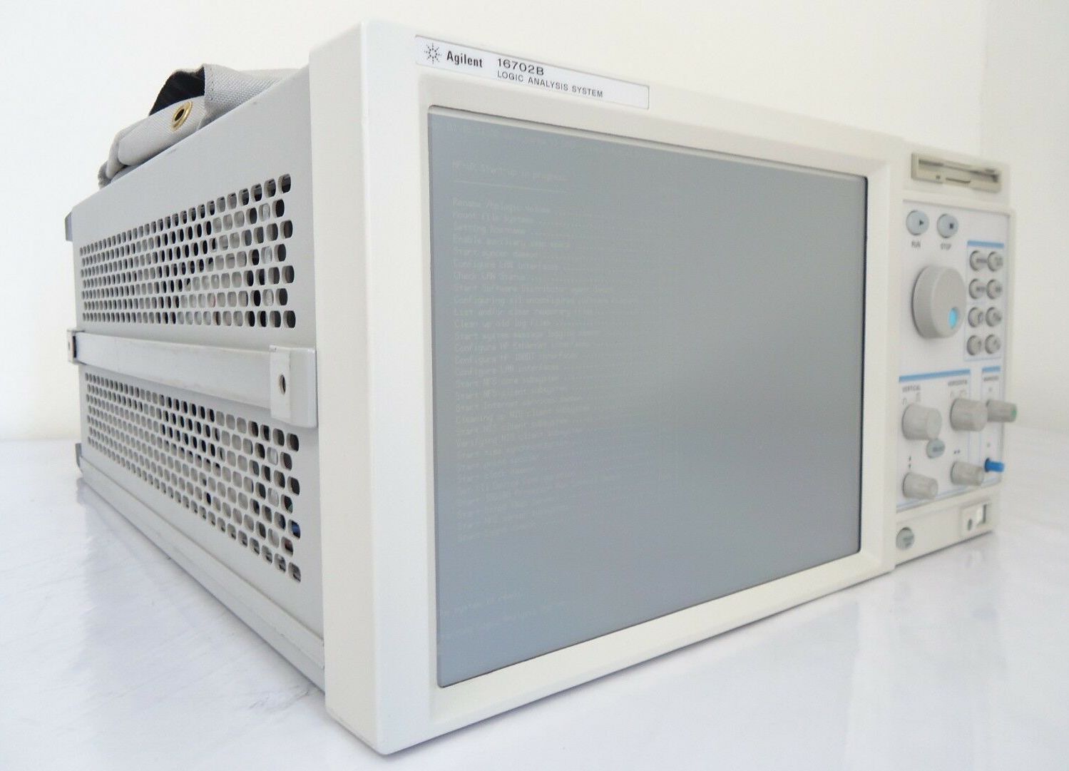
This thing is seriously awesome. It has big ol knobs that feel amazing to spin around, a surprisingly good touch screen, and, best of all… a floppy drive. This is a seriously massive unit, and weighs close to 35 pounds, and works quite well as a space heater as well. In the back of the unit, there’s a few slots that you can insert different cards into: my unit came with two 16718A cards, which allow state analysis at up to 333MHz; each card provides 72 channels.
Despite being close to 20 years old, this thing definitely can still hold its own. With the Ethernet port on the back, you can remote control this thing – and, since the OS on this analyzer is just a modified HP-UX, it’s pretty simple to use X11 forwarding to use the analyzer from the comfort of your slightly more modern computer.
Putting it to the Test
I justified getting this analyzer in my head because it would make debugging the hardware of a hypothetical 68000-based computer that I’ve wanted to design and build for years a lot easier. Obviously, now that I have this analyzer, that hardware should become more than an idea in my head, but I digress… it’s only fitting that we’re going to go use the 68000’s little brother, the 68008, free running to put this analyzer to the test.
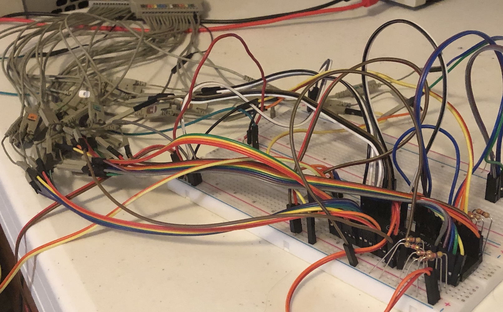
On the breadboard, we have a 68008, a 2MHz oscillator, and some pull-downs to make the data bus read $00, the opcode for ORI.B #0, D0. You’ll also need to pull up at least RESET, BR, and tie DTACK low.
Sample Clocks
At this point, you could connect a LED to one of the higher address lines (like A15) and watch it blink away happily, but that’s not why we’re here. I only had one cable, so I was limited to two pods, aka a “measly” 32 channels. That, however, is enough to get most all CPU control lines, the complete data bus, and the low 16 bits of the address bus captured.
From the workspace screen, you can get to the detail page for each of the boards installed in your system. There, you can assign the pods, configure clocks, and most importantly, assign labels to the signals. Let’s start on the first tab, the Sampling screen.
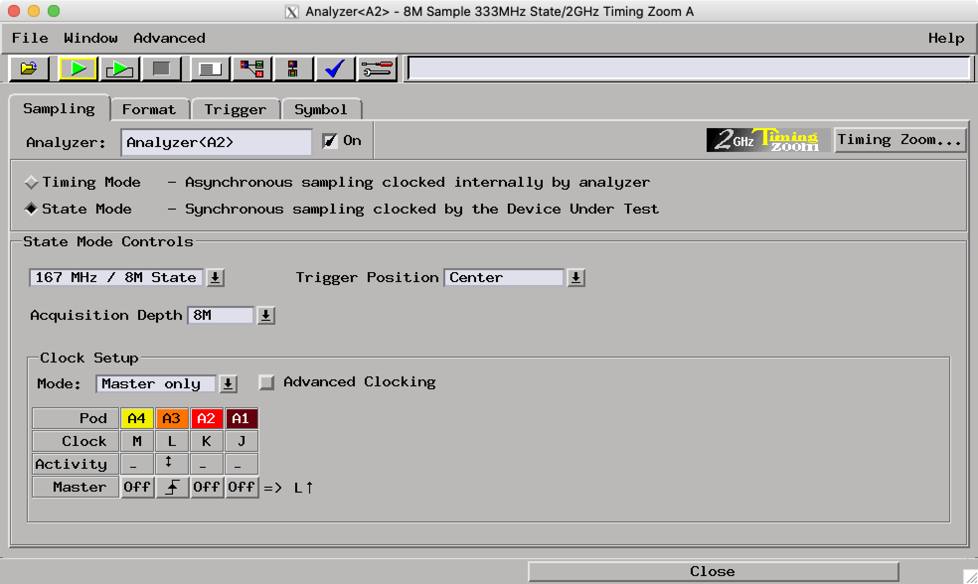
In this case, I’ve chosen to use the State mode – in this mode, we have to feed a clock into the analyzer, and it will sample our inputs every time that clock cycles. You could just as well use Timing mode, but you can fit a lot more data into the sample buffer in State mode, at the cost of less timing resolution.
At the bottom of the window, I’ve configured the rising edge of the L clock on Pod 3 to be when we sample signals. You can have it trigger on either edge, or even use multiple different clocks. The little Activity section will show you the state of that clock, which is very convenient.
Signals & Labels
Next up, let’s assign labels to our signals to make our analysis make more sense. The interface is pretty self-explanatory, aside from the fact that you right-click on an existing label to create a new one. Meh.
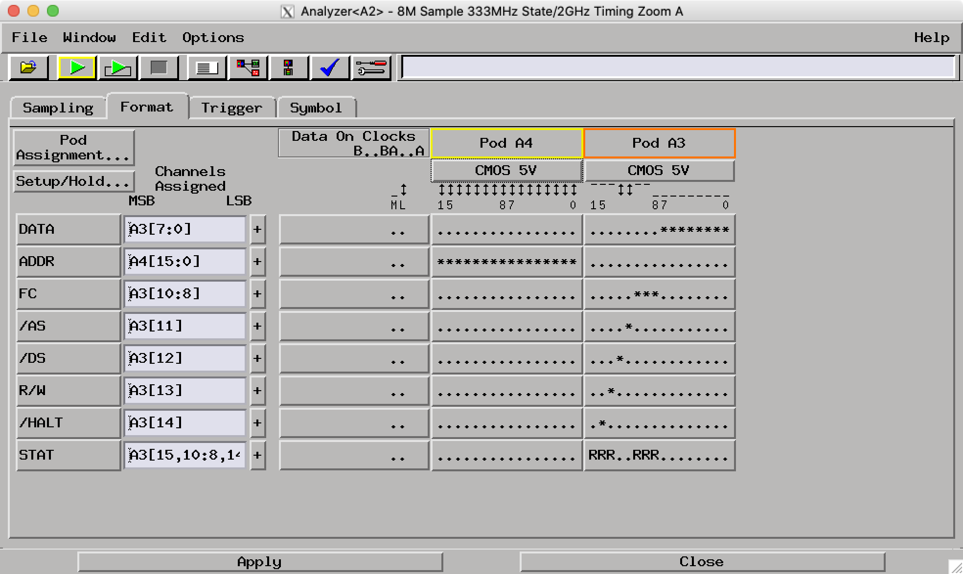
You can also configure the IO standard in use – click the buttons right underneath the pod names to do that. Since this is a CMOS 68008, it’s set to CMOS 5V, but TTL would work just as well. A neat feature to point out is again, the state of the individual lines is displayed at the top of the table, underneath the IO standard.
Most of those signals should make sense if you’re familiar with the 68000 bus, but the STAT label might stand out – this is used by the inverse assembler to get info on CPU state to properly decode the bus states. More on those later.
Configuring Triggers
One of my favorite features about this analyzer is how powerful the triggering functionality is. Head on over to the Trigger tab, and you’ll see exactly what I mean.
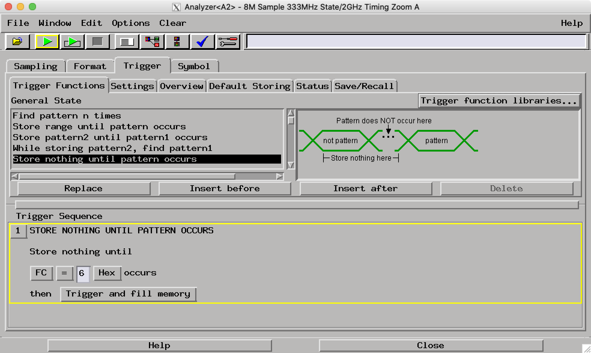
There’s quite a few trigger functions to chose from, and you can actually chain them one after another. This is some super powerful stuff: you could use this to trigger, for example, on the 5th access to a particular address in a row, or something like that. But instead, I just wait for a CPU space cycle on startup to start my sampling. You could also look for the falling edge of AS, if you give it a weak pull up, for example.
Capturing Data
Once you’ve set up the triggers, you can hit the green triangle button in the toolbar to start a capture. The first one will trigger once, then capture data; while the second will do so continuously. After the capture is complete, there’s a few options on viewing the data you captured:
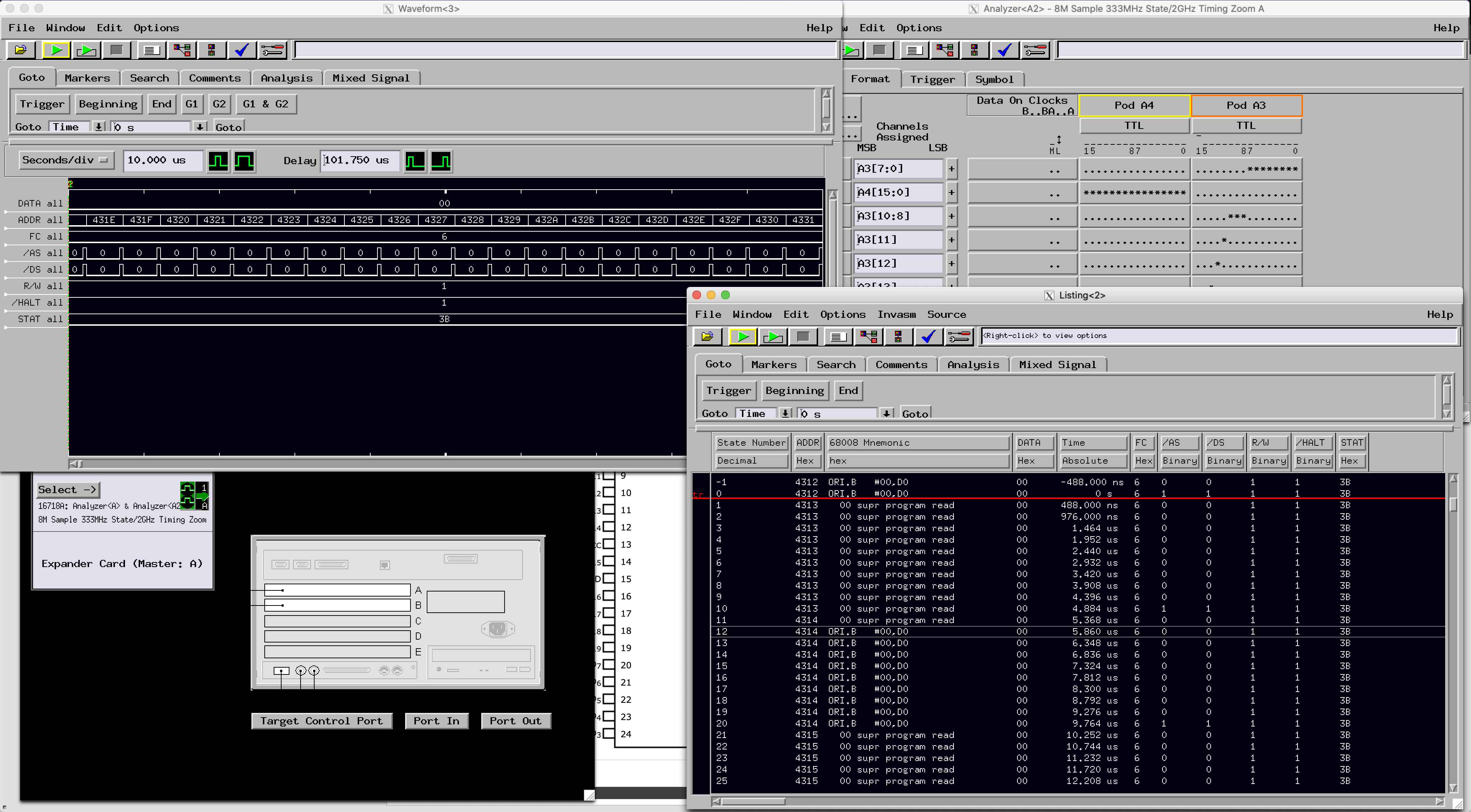
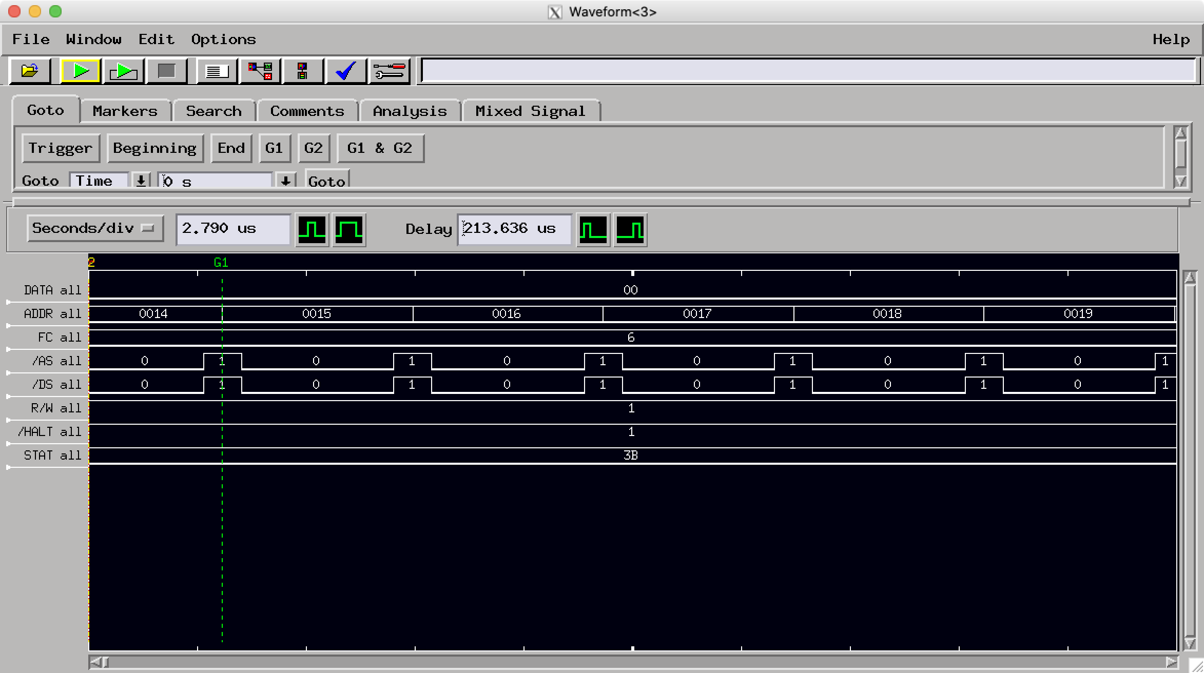
Waveform
This is the view of a logic analyzer you’re probably most familiar with, especially if you’ve ever used Saleae’s excellent software. All labels are displayed, and you can do some basic searching for values.
Listing
The alternative is the listing view – something you’re familiar with if you’ve ever used this machine, or any of the other 16xxx series logic analyzers, and this is probably my favorite feature of this machine.
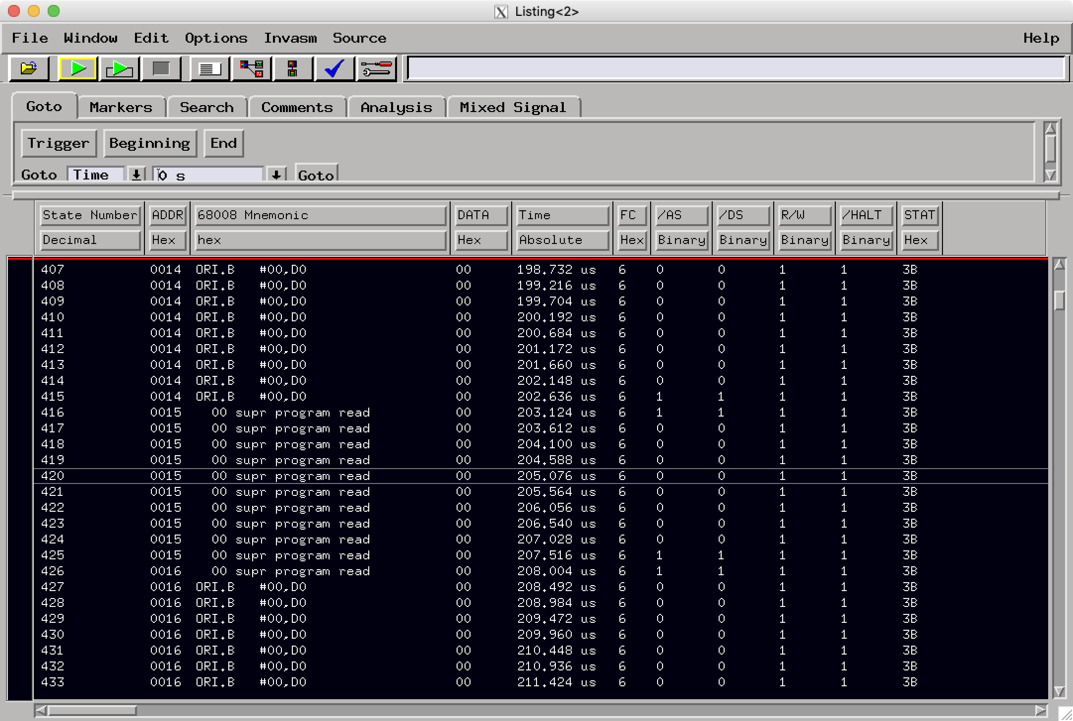
You’ll notice the “68008 Mnemonic” column: this is a column added by an inverse assembler – a little piece of code that interprets your captured data, and decodes things such as bus transactions, and in this case, even shows a disassembly of the exact instruction fetched by the processor.
This is super convenient because here, we see ORI.B #0, D0 – this is exactly the instruction we wanted to put on the bus by pulling it down to $00. This feature can also be used in conjunction with a source listing, but I haven’t yet figured out how to use that feature. Supposedly, this will allow you to correlate your captured data to your source code, which sounds pretty neat.
You can also save this data to the analyzer’s internal disk, and presumably consume it in other software. I haven’t yet tried this either, but considering the analyzer can mount NFS shares, being able to save data to a fast NFS share would be a great ability to have. (Well… as fast as it could be over 100Mbps Ethernet, but meh.)
Inverse Assemblers
My machine didn’t have the inverse assemblers installed by default, so I had to download them. This forum thread has some downloads and more information on how they work.
As mentioned earlier, some of these analyzers require additional bus signals, which are usually collected under a STAT label. Specifically, this post has a version of the inverse assemblers that comes with some description files; those don’t explicitly state what bit in STAT does what, but you can usually figure it out pretty easily with some intuition.
Once you’ve loaded and installed the inverse assemblers onto your device (FTP as root is easiest, then load them using the File Manager) you can assign one through the Invasm menu in the Listing window.
X11 Forwarding
Getting the logic analyzer application to run once you’ve configured X11 forwarding is pretty straightforward. Log in as the hplogicz user via telnet, configure the DISPLAY environment variable (this will be something like 172.16.2.2:0.0, of course replacing the IP of your machine) and then running vp &.
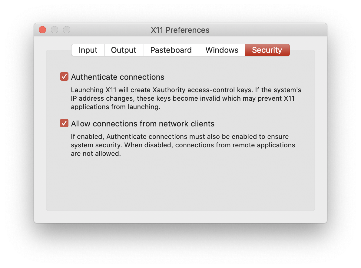
I would keep getting “connection refused by server” errors on the telnet session – I figured it would be easier to get this working on a Mac (albeit with the “semi native” XQuartz) than on Windows, but that proved to not be the case. Thankfully, once I did some research, the fix was pretty simple. X11 on macOS needs to be configured to allow remote connections. Fire up the XQuartz preferences, and change the following settings:
If you’re brave, you can try and get everything working with XAuthority files and all that good stuff to keep things secure, but I ended up just connecting the analyzer directly to my machine via an extra Ethernet port, and ran xhost + on my machine to allow X11 connections from anywhere. (Do note that this is incredibly insecure: I have the firewall on my machine configured to only allow connections to the X server via that dedicated Ethernet interface!)
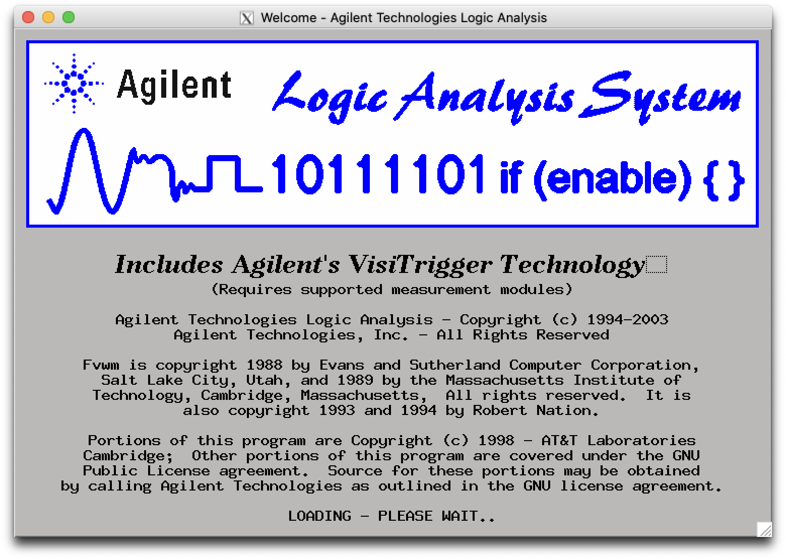
Once you’ve done this, repeat the above sequence of commands, and you should be greeted with this lovely splash screen that’s peak 1990s UI design.
Resources
It can be a bit tricky to get these machines to cooperate. Thankfully, I didn’t have to do a whole lot besides plugging it in, but here’s a few pages I found handy in getting everything set up:
- These threads on the EEVblog forums contain plenty of great information about how to set this machine up. Licenses for basically all “tool sets” are available online, and you can get root access to the underlying HP-UX install and modify the analyzer to your heart’s content.
- Matt Millman’s 16702B page had some information on how to get the X11 forwarding working. You’re supposed to be able to just log in with the
logicuser, but that didn’t work for me, as described above.